The Neural Network Odyssey: Core Concepts to Code, Part 2
Diving into Data Flow and Learning Algorithms with an Introductory PyTorch Tutorial
Introduction to Neural Networks - Deepening Our Understanding
Welcome Back to the World of Neural Networks
Last week, in Part 1 of our exploration into neural networks, we embarked on a fascinating journey to understand these powerful tools that are reshaping the landscape of artificial intelligence. We delved into the biological inspirations behind neural networks, uncovering how the human brain's intricate network of neurons and synapses has inspired a revolution in computing. We navigated through the basics of artificial neurons, discussing the structure of perceptrons, and the pivotal role of weights and biases in this architecture. Our exploration also took us through the various layers of a neural network, highlighting how each layer contributes to the complex task of pattern recognition and decision-making.
As we progressed, we uncovered the importance of activation functions, learning about their types and purposes in the context of a neural network. These functions, acting as gatekeepers, determine the output of a neural network, influencing its ability to learn and make accurate predictions. Today, in Part 2 of our series, we're going to deepen our understanding of neural networks. We'll explore how data moves through these networks in a process called forward propagation and unravel the mysteries of backpropagation, a key component in teaching neural networks to learn from their mistakes. Additionally, we will step into the practical world, where we will implement a basic neural network using PyTorch, marking our transition from theory to application.
This part of our journey is crucial as it bridges the gap between understanding the components of neural networks and seeing them in action. By the end of this section, you'll have a firmer grasp on how neural networks function and how they are trained, setting the stage for more advanced topics in the coming weeks. So, let's dive in and continue our adventure into the intricate and fascinating world of neural networks.
Forward Propagation
Understanding Forward Propagation
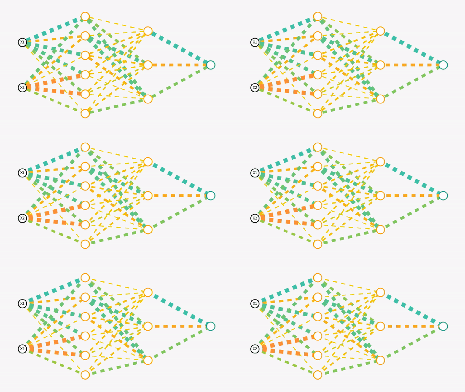
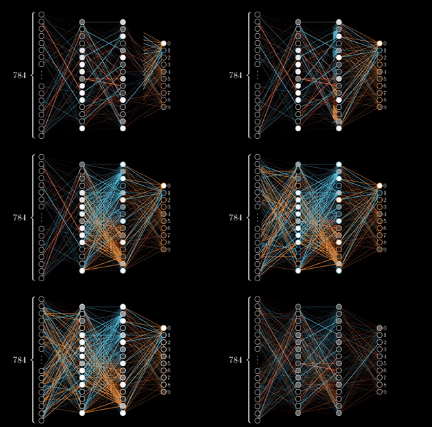
Forward propagation is the process by which a neural network makes sense of the input data, transforming it through various layers to produce an output. Imagine it as a journey where the data travels through the network, getting transformed at every step before reaching its final destination, the output layer.
The Journey of Data in a Neural Network
The Starting Point: Input Layer
The input layer is where the journey begins. Each neuron in this layer represents a feature of the input data. For instance, in an image recognition task, each neuron might correspond to a pixel's intensity in the image.
Moving Through Hidden Layers
After the input layer, data moves to one or more hidden layers. These layers are the network's decision-making body. Each neuron here receives data from all neurons in the previous layer, processes it, and passes it on. This is where the magic of neural networks truly happens.
Weights and Biases: The Modifiers
As data travels from one neuron to another, it gets modified by weights and biases. Think of weights as the influence one neuron has over another. A higher weight means more influence. Biases, on the other hand, are like the neuron’s personal opinion, adjusting the output regardless of the input.
Activation Functions: The Decision Makers
Each neuron processes the weighted sum of its inputs and then applies an activation function. Activation functions decide how much of this signal should be passed forward. Common examples include the Sigmoid, Tanh, and ReLU functions. These functions introduce non-linearity, allowing the network to handle complex patterns.
The Role of Activation Functions
Activation functions play a crucial role in forward propagation. Without them, the neural network would just be performing a series of linear transformations. Non-linearity introduced by activation functions allows neural networks to learn from and model complex data such as images, audio, and nonlinear relationships.
The Final Destination: Output Layer
After traversing through the hidden layers and undergoing multiple transformations, the data reaches the output layer. The structure of this layer depends on the type of problem. For instance, in classification tasks, this layer often uses a Softmax function to interpret the neural network's final output as probabilities.
The Essence of Forward Propagation
In essence, forward propagation is a well-choreographed sequence of linear and nonlinear transformations. These transformations are dictated by the network’s architecture (number of layers and neurons), weights, biases, and activation functions. The output of forward propagation is then used for prediction and further compared with the actual result to improve the network during backpropagation.
Forward propagation is the neural network's way of 'thinking' and making sense of the input data. By understanding this process, one can gain insights into how neural networks learn and make decisions, forming a foundational understanding for more complex topics in neural network training and optimization.
Understanding Backpropagation
Backpropagation stands as one of the most pivotal mechanisms in training neural networks, allowing them to refine their predictions and improve accuracy over time. At its core, backpropagation is a method for updating the weights in a neural network in a way that minimizes the difference between the predicted output and the actual output.
The Concept of Learning in Neural Networks
To understand backpropagation, it's crucial to first grasp how neural networks learn. A neural network's goal is to make predictions or classifications as accurately as possible. During the training phase, the network makes a prediction, and then it needs to measure how far off this prediction is from the actual result. This measure of error is encapsulated in what we call a 'loss function' or 'cost function.'
The Role of Loss Functions
The loss function quantifies the difference between the network's prediction and the actual output. Common examples include the Mean Squared Error (MSE) for regression tasks and Cross-Entropy for classification tasks. The value of this loss function is what the network aims to minimize during training.
The Essence of Backpropagation
Backpropagation is essentially a practice of reverse engineering the error. It starts at the output layer, where the network's prediction and the actual value are compared, and then traces back through the network's layers, calculating the error gradient at each step. This process involves two key mathematical concepts: the chain rule from calculus and partial derivatives.
By applying the chain rule, the backpropagation algorithm efficiently computes the gradient of the loss function with respect to each weight in the network. This gradient tells us in which direction we should adjust our weights to minimize the error.
Gradient Descent: Adjusting the Weights
The gradients calculated during backpropagation are then used to update the weights of the network. This is where the concept of 'gradient descent' comes in. Imagine you're at the top of a hill and your objective is to reach the lowest point. At each step, you look around to find the steepest descent and take a step in that direction. In neural networks, each step represents an iteration of weight adjustment, and the size of the step is determined by the learning rate, a hyperparameter that controls how much we adjust the weights

Learning Rate: A Delicate Balance
The learning rate is crucial: too high, and the network might overshoot the optimal point; too low, and it could take too long to converge or get stuck in a local minimum. This rate can be adjusted as training progresses, a technique known as learning rate annealing or adaptive learning rates.
Putting It All Together
In each training iteration (or epoch), the entire dataset is passed through the network, predictions are made, errors are calculated, and backpropagation is used to adjust the weights. This process repeats until the network's performance stops improving, or other stopping criteria are met.
In summary, backpropagation is an elegantly powerful mechanism that enables neural networks to learn from their mistakes, adjusting and improving with each iteration. It's a foundational concept in neural networks, enabling them to tackle complex, real-world problems with increasing accuracy and efficiency.
Neural Network Code with PyTorch
Let's create a simple binary classification neural network using PyTorch. This example will use a synthetic dataset for ease of understanding. The network will be a basic feedforward architecture with one hidden layer. We'll use the ADAM optimizer and binary cross-entropy loss, as you requested.
First, ensure you have PyTorch installed. If not, you can install it via pip:
pip install torch torchvisionNow, let's dive into the code:
Importing Necessary Libraries
import torch
import torch.nn as nn
import torch.nn.functional as F
import torch.optim as optim
from sklearn.datasets import make_classification
from sklearn.model_selection import train_test_split
from torch.utils.data import DataLoader, TensorDataset
Creating a Synthetic Dataset
# Generate a synthetic binary classification dataset
X, y = make_classification(n_samples=1000, n_features=20, n_classes=2, random_state=42)

# Convert to PyTorch tensors
X_tensor = torch.tensor(X, dtype=torch.float32)
y_tensor = torch.tensor(y, dtype=torch.float32)

# Split the dataset into training and testing sets
X_train, X_test, y_train, y_test = train_test_split(X_tensor, y_tensor, test_size=0.2)

# Create DataLoader for both training and testing
train_data = DataLoader(TensorDataset(X_train, y_train), batch_size=64, shuffle=True)
test_data = DataLoader(TensorDataset(X_test, y_test), batch_size=64, shuffle=False)
Defining the Neural Network
class BinaryClassifier(nn.Module):
    def __init__(self):
        super(BinaryClassifier, self).__init__()
        self.fc1 = nn.Linear(20, 10)  # 20 input features, 10 outputs to hidden layer
        self.fc2 = nn.Linear(10, 1)   # 10 inputs from hidden layer, 1 output (binary classification)

    def forward(self, x):
        x = F.relu(self.fc1(x))      # Activation function for hidden layer
        x = torch.sigmoid(self.fc2(x))  # Sigmoid activation for output
        return x

# Create an instance of the network
model = BinaryClassifier()
Setting up the Optimizer and Loss Function
optimizer = optim.Adam(model.parameters(), lr=0.001)
loss_function = nn.BCELoss()
Training the Network
# Number of epochs
epochs = 5

for epoch in range(epochs):
    model.train()
    for inputs, labels in train_data:
        optimizer.zero_grad()  # Clear gradients from the last step
        outputs = model(inputs)
        loss = loss_function(outputs.squeeze(), labels)
        loss.backward()  # Compute gradients
        optimizer.step()  # Update weights

    print(f'Epoch {epoch+1}/{epochs}, Loss: {loss.item():.4f}')
Evaluating the Model
model.eval()  # Set the model to evaluation mode
with torch.no_grad():  # Turn off gradients for validation
    correct = 0
    total = 0
    for inputs, labels in test_data:
        outputs = model(inputs)
        predicted = (outputs.squeeze() > 0.5).float()  # Convert probabilities to class labels
        total += labels.size(0)
        correct += (predicted == labels).sum().item()

accuracy = 100 * correct / total
print(f'Accuracy: {accuracy:.2f}%')
This code sets up a simple binary classifier using PyTorch. It creates a synthetic dataset, defines a neural network model, trains this model, and evaluates its accuracy. Remember, this is a basic example for illustrative purposes. Real-world applications would require more complex architectures, data preprocessing, and hyperparameter tuning.
Conclusion
As we wrap up our exploration into the foundational aspects of neural networks, we've journeyed from the conceptual understanding of how data moves through layers and nodes, to the critical process of learning via backpropagation and gradient descent. With these concepts in hand, you're now equipped with the knowledge to build and train basic neural networks. Looking ahead, next week promises to be an exciting venture as we delve into Convolutional Neural Networks (CNNs). A cornerstone in the field of image recognition and analysis, CNNs represent a fascinating leap from the general structure of neural networks to more complex and powerful models, opening doors to a myriad of applications in the real world. Join us as we unfold the layers of CNNs, understanding how they mimic the human visual system and revolutionize the way machines interpret images.
References:
PyTorch Documentation: https://pytorch.org/docs/1.13/


