
From Pixels to Patterns
Exploring CNN Architectures and Image Recognition using PyTorch


Introduction
Welcome back to our journey through the fascinating world of Convolutional Neural Networks (CNNs)! Last week, in Part 1, we laid the foundation by exploring the basic concepts and components of CNNs. We jumped into the essence of convolutional layers, understood the significance of filters or kernels, and touched upon the critical role of activation functions, particularly ReLU, in these networks.

This week, in Part 2, we're going to dive deeper. Our exploration will take us into the intricate workings of pooling layers and their role in CNN architectures. We'll see how these layers contribute to the network's ability to process and understand images effectively.
But that's not all. We'll also piece together everything we've learned so far by looking at a basic CNN architecture using PyTorch. Understanding this architecture is key to grasping how CNNs are able to achieve remarkable feats in fields like image recognition.
Stay tuned, as what you learn here will not only deepen your knowledge but also equip you with insights that are crucial for any aspiring AI expert!
Pooling Layers in Convolutional Neural Networks (CNNs)
Defining Pooling in CNNs: Pooling, also known as subsampling or downsampling, is a critical component in CNNs. Its primary function is to progressively reduce the spatial size of the representation, thus reducing the number of parameters and computation in the network. This not only helps in controlling overfitting but also ensures that the network becomes increasingly invariant to small transformations, distortions, and translations in the input data.
Types of Pooling:
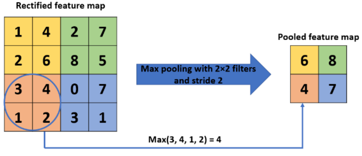
Max Pooling: This is the most common form of pooling, where the maximum value from a set of values in the filter size is selected. For instance, in a 2x2 filter, max pooling will take the largest value out of the 4 values in the filter. This method is effective in capturing the most significant features like edges, textures, etc.
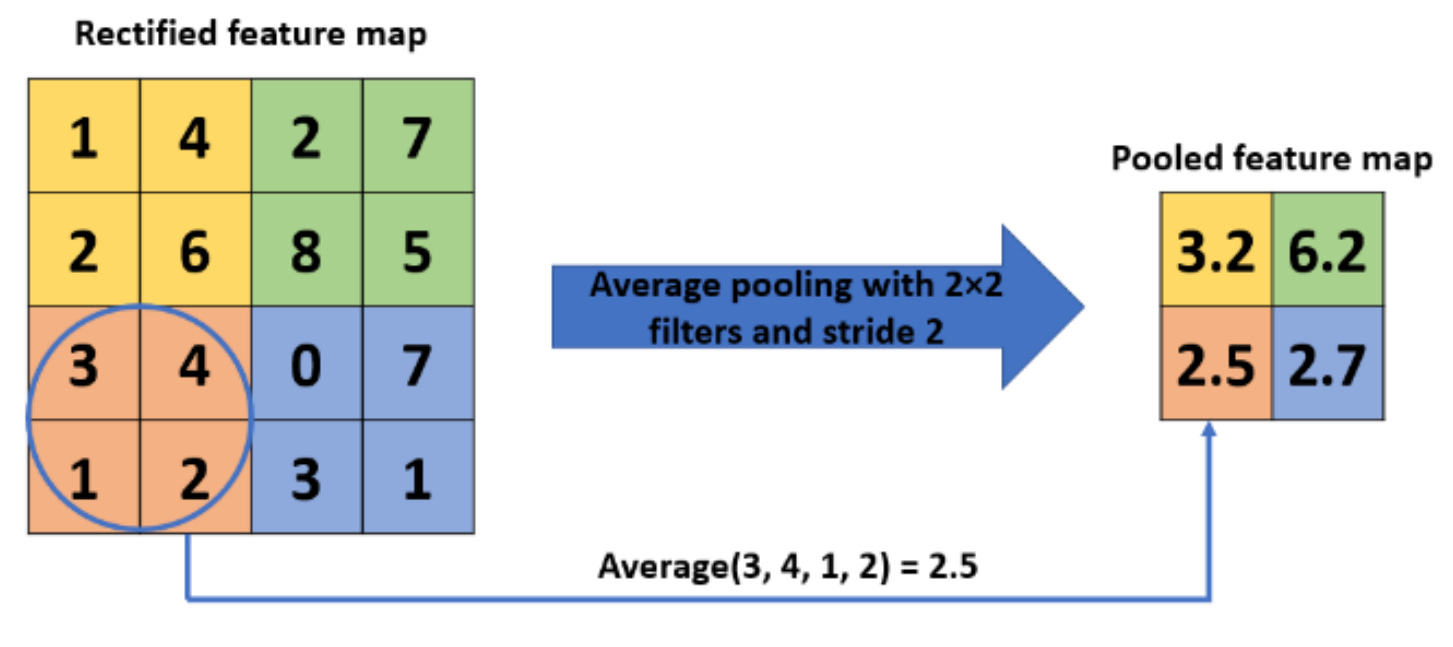
Average Pooling: As the name suggests, this approach takes the average of all the values in the filter size. It calculates the average for each subregion of the input. While max pooling tends to select the brightest pixels from the image, average pooling provides a smoother and more subdued representation.
The Process of Pooling:
In pooling, a filter (usually of size 2x2 or 3x3) moves across the input data (the output from the previous layer, typically a convolutional layer) with a specified stride (the amount by which the filter moves).
At each position, the filter covers a portion of the input and performs the max or average operation, depending on the pooling type.
This process reduces the dimensionality of the data, allowing the network to focus on the most prominent features and making it less sensitive to the exact location of features in the input.
Why is Pooling Important?
Dimensionality Reduction: Pooling significantly reduces the number of parameters and computations in the network, thus reducing the computational cost and the risk of overfitting.
Feature Representation: It helps in achieving a form of translation invariance. For example, after pooling, the exact location of a feature becomes less critical. This is crucial for tasks like image recognition, where we care more about whether a feature is present rather than its exact location.
Robustness to Variations: By summarizing the features in a region, pooling helps the network to be robust to small variations, noise, and distortions in the input.
Considerations in Using Pooling:
Choice of Pooling Type: Max pooling is a go-to choice in many scenarios for its effectiveness in feature extraction. However, average pooling can sometimes be useful, especially in cases where the smoothness of the feature map is desired.
Filter Size and Stride: These parameters define how much the pooling operation will reduce the dimensions of the input data. A larger filter and stride will result in more significant downsampling.
Pooling is a simple yet powerful concept in CNNs. By reducing the spatial size of the feature maps, pooling layers play a pivotal role in ensuring that CNNs can abstract higher-level features from the input data while keeping the computational load manageable. This efficiency makes them indispensable in complex architectures designed for tasks ranging from image and video recognition to medical image analysis.
Building a Basic CNN Architecture with PyTorch
In this section, we'll walk through how to build a basic CNN using PyTorch. We'll create a simple model suitable for classifying images. Before diving into the code, ensure you have PyTorch installed in your environment.
Setting Up
First, import the necessary libraries:
import sys
import torch
import torch.nn as nn
import torch.optim as optim
import torchvision
from torchvision import datasets, transforms
from torch.utils.data import DataLoader
from sklearn.metrics import accuracy_score
import matplotlib.pyplot as plt
import numpy as np
Next, let's perform a check to utilize the GPU if it's available:
# Check if GPU is available and set the device accordingly
Device = torch.device('cuda:0' if torch.cuda.is_available() else 'cpu')
n_gpu = torch.cuda.device_count()
print(f'Using device: {torch.cuda.get_device_name(0)}')

Output (something similar to):

Using device: NVIDIA GeForce RTX 4090
Preparing the Dataset
We'll use a standard dataset like MNIST, which consists of handwritten digits. PyTorch makes it easy to load and preprocess datasets:
# Transformations applied on each image
transform = transforms.Compose([
    transforms.ToTensor(),  # Convert images to PyTorch tensors
    transforms.Normalize((0.5,), (0.5,))  # Normalizing the images
])

# Loading the training dataset
train_dataset = datasets.MNIST(root='./data', train=True, download=True, transform=transform)
train_loader = DataLoader(train_dataset, batch_size=64, shuffle=True)

# Loading the test dataset
test_dataset = datasets.MNIST(root='./data', train=False, download=True, transform=transform)
test_loader = DataLoader(test_dataset, batch_size=64, shuffle=False)
Let’s visualize some of the training images:

Defining the CNN Architecture
Now, let's define our CNN architecture. We'll create a simple network with two convolutional layers followed by two fully connected layers.
In our CNN architecture, we use two convolutional layers followed by two fully connected layers, a setup well-suited for tasks like image classification on the MNIST dataset. The convolutional layers are crucial for extracting varying levels of features from the images, with the first layer picking up basic attributes like edges and the second layer building upon these to recognize more complex features. Following these, the fully connected layers interpret these extracted features, culminating in the output layer that classifies the images into distinct categories. This configuration strikes a balance between complexity and efficiency, making it capable of capturing and analyzing essential patterns in the data while avoiding overfitting, a common concern with more intricate networks.
class SimpleCNN(nn.Module):
    def __init__(self):
        super(SimpleCNN, self).__init__()
        self.conv1 = nn.Conv2d(1, 32, kernel_size=3, stride=1, padding=1)
        self.conv2 = nn.Conv2d(32, 64, kernel_size=3, stride=1, padding=1)
        self.fc1 = nn.Linear(7*7*64, 128)
        self.fc2 = nn.Linear(128, 10)

        self.relu = nn.ReLU()
        self.pool = nn.MaxPool2d(2, 2)
        self.dropout = nn.Dropout(0.5)

    def forward(self, x):
        x = self.pool(self.relu(self.conv1(x)))
        x = self.pool(self.relu(self.conv2(x)))
        x = x.view(-1, 7*7*64)  # Flatten the tensor for the fully connected layer
        x = self.relu(self.fc1(x))
        x = self.dropout(x)
        x = self.fc2(x)
        return x

model = SimpleCNN().to(device)
print(model)

Output:

SimpleCNN(
  (conv1): Conv2d(1, 32, kernel_size=(3, 3), stride=(1, 1), padding=(1, 1))
  (conv2): Conv2d(32, 64, kernel_size=(3, 3), stride=(1, 1), padding=(1, 1))
  (fc1): Linear(in_features=3136, out_features=128, bias=True)
  (fc2): Linear(in_features=128, out_features=10, bias=True)
  (relu): ReLU()
  (pool): MaxPool2d(kernel_size=2, stride=2, padding=0, dilation=1, ceil_mode=False)
  (dropout): Dropout(p=0.5, inplace=False)
)
Model Training
Next, we'll define our loss function and optimizer, and train the model:
criterion = nn.CrossEntropyLoss()
optimizer = optim.Adam(model.parameters(), lr=0.001)

# Training loop
for epoch in range(5):  # 5 epochs
    for i, (images, labels) in enumerate(train_loader):
        images, labels = images.to(device), labels.to(device)  # Move data to the device

        # Forward pass
        outputs = model(images)
        loss = criterion(outputs, labels)

        # Backward pass and optimization
        optimizer.zero_grad()
        loss.backward()
        optimizer.step()

        if (i+1) % 100 == 0:
            print(f'Epoch [{epoch+1}/5], Step [{i+1}/{len(train_loader)}], Loss: {loss.item():.4f}')

Output:

Epoch 05/05, Batch 938 | Loss: 0.00   | Tr Acc: 100.00%
CPU times: total: 1.64 s
Wall time: 37.6 s
Test Model Performance
# Ensuring the model is in evaluation mode
model.eval()

y_test, y_pred = [], []
for images, labels in test_loader:
    images, labels = images.to(device), labels.to(device)
    y_test.extend(labels.cpu().numpy())

    with torch.no_grad():
        outputs = model(images)
        _, predicted = torch.max(outputs.data, 1)
        y_pred.extend(predicted.cpu().numpy())

# Calculate accuracy
accuracy = accuracy_score(y_test, y_pred)
print(f'Accuracy of the model on the test images: {accuracy * 100:.2f}%')

Output:

Accuracy of the model on the test images: 99.23%
View Predicted Images
# View some predicted images
import matplotlib.pyplot as plt
import numpy as np

fig = plt.figure(figsize=(10, 10))
columns = 4
rows = 5
for i in range(1, columns*rows + 1):
    img_xy = np.random.randint(len(test_dataset))
    img = test_dataset[img_xy][0][0,:,:]
    fig.add_subplot(rows, columns, i)
    plt.title(f'Predicted: {y_pred[img_xy]}, Label: {y_test[img_xy]}')
    plt.axis('off')
    plt.imshow(img, cmap='gray')
plt.show()
In this exploration with a simple CNN model, we achieved an exceptional accuracy rate of over 99% on the MNIST dataset. This result not only underscores the robustness and effectiveness of Convolutional Neural Networks in image recognition tasks but also reflects the high quality and well-structured nature of the MNIST dataset, making it an ideal benchmarking tool in the realm of machine learning. While this high level of accuracy is certainly encouraging, it opens avenues for further exploration and experimentation. It paves the way for applying similar methodologies to more complex and realistic image recognition challenges, beyond the somewhat idealized confines of MNIST. With that said, it's important to remain mindful of other critical aspects such as the model's generalization capability, its performance on diverse and noisy datasets, and computational efficiency. This success serves as a promising stepping stone and a testament to the potential of CNNs in the broader spectrum of computer vision applications, inspiring us to delve deeper into this fascinating domain.
Conclusion
In this second part of our exploration into Convolutional Neural Networks, we went deeper into the intricacies of CNN architecture, focusing on pooling layers and their vital role in reducing computational complexity and extracting dominant features. We also pieced together the elements of a basic CNN architecture, emphasizing its significance in practical applications, particularly in image recognition. This journey through the foundational aspects of CNNs equips you with a clearer understanding of how these powerful networks operate and their remarkable ability to interpret and analyze visual data. As we wrap up this segment, we set the stage for future discussions that will take us into more advanced territories of CNNs and their diverse applications, opening doors to a world where artificial intelligence not only sees but also understands its surroundings with ever-increasing sophistication.
GitHub Code
If you’d like to explore the code further, feel free to check out the Jupyter Notebook on GitHub.
Me podes a yudar
Hola