Advanced Strategies for Superior Supervised Models
How to Fine-Tune Performance with Ensemble, Regularization, and Data Balancing Techniques
Introduction
In this week's post, we dive deeper into the realm of advanced supervised learning techniques that push the envelope beyond traditional models. After covering the foundational elements, practical implementations, and fine-tuning methods in our previous discussions, we now turn our focus toward techniques designed to amplify model performance further. From ensemble methods to regularization, these approaches not only enhance your model's predictive capabilities but also offer practical solutions to tackle challenges such as overfitting and imbalanced datasets.
Our exploration begins with a detailed look at ensemble methods, which amplify predictive power by combining the outputs of multiple models. We then move on to discuss regularization techniques designed to keep your models from overfitting the training data. Additionally, we will address strategies for effectively handling imbalanced datasets, a prevalent but frequently neglected issue in real-world machine learning applications. This week's material aims to arm you with advanced tools and techniques that could redefine the performance and utility of your supervised learning models.
Ensemble Methods
Ensemble methods are an integral part of advanced supervised learning techniques, offering a powerful way to improve model performance. The core idea is simple yet effective: instead of relying on a single model to make predictions, why not consult a "committee" of models and have them vote on the outcome? In this section, we'll delve into the main types of ensemble methods, namely Bagging, Boosting, and Stacking, to see how they work and why they are valuable tools in a data scientist's repertoire.
Bagging
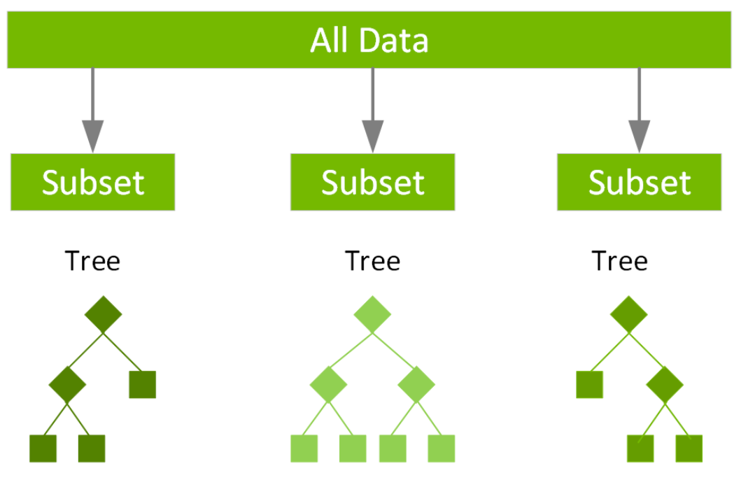
Bootstrap Aggregating, commonly known as Bagging, is one of the earliest ensemble methods. In Bagging, we train multiple instances of the same model on different subsets of the training data. These subsets are created by randomly sampling the original dataset with replacement. After training, each model gets to vote, and the final prediction is typically an average (for regression problems) or a majority vote (for classification problems).
The primary advantage of Bagging is its ability to reduce overfitting. By training different models on varied subsets of the data, Bagging lessens the chance that the ensemble will memorize the noise in the training set, leading to a more robust model.
Popular algorithms that utilize Bagging include Random Forests, which extend the Bagging concept to Decision Trees by also selecting a random subset of features at each split.

Boosting
While Bagging aims to train independent models in parallel, Boosting takes a different approach by training models sequentially, with each model trying to correct the errors of its predecessor. Algorithms like AdaBoost and Gradient Boosting are the poster children for this technique. In AdaBoost, each data point is assigned a weight, and these weights are adjusted between rounds (i.e., each training iteration of a new model in the ensemble) to focus more on the examples that the previous model got wrong.
Boosting is powerful but comes with the risk of overfitting, especially if the base models are too complex or if the ensemble contains too many models. Therefore, it's often crucial to include some form of regularization, such as limiting the depth of the base decision trees or using a learning rate to temper the adjustments made at each round.
Stacking
Stacking, or Stacked Generalization, is a more sophisticated ensemble technique that combines multiple different types of models. Unlike Bagging and Boosting, which often use the same kind of base model, Stacking can integrate various machine learning algorithms like k-NN, SVM, or Neural Networks.
In Stacking, each model is trained independently on the full training set. Their predictions are then used as inputs for a "meta-model," which is trained to make the final prediction. The idea is to leverage the strengths of each individual model to produce a final prediction that is more accurate and robust than any single model could achieve on its own.
The art of Stacking lies in selecting the right base models and the right meta-model. It's often advised to use models that have diverse strengths and weaknesses so that they complement each other.
Regularization Techniques in Supervised Learning
Regularization techniques are a crucial part of machine learning models, especially in supervised learning, where the risk of overfitting is high. Overfitting happens when a model learns the noise in the training data to the point that it negatively impacts the performance of the model on new, unseen data. Essentially, the model becomes too tailored to the training data and loses its ability to generalize. Regularization techniques help to constrain the optimization process during training, discouraging complex models that overfit the data.
L1 Regularization (Lasso)
L1 Regularization, commonly known as Lasso (Least Absolute Shrinkage and Selection Operator), adds a penalty term to the cost function equal to the absolute value of the magnitude of the coefficients. Mathematically, the cost function J(θ) for L1 regularization can be written as:
Here, λ is the regularization parameter, and ∣∣θ∣∣1 denotes the L1 norm of the model parameters. By doing so, L1 has the effect of setting some of the less important features' coefficients to zero, effectively ignoring them, and thereby creating a more parsimonious model. This characteristic makes L1 regularization useful for feature selection in cases where we have a large number of features.
L2 Regularization (Ridge)
L2 Regularization, also known as Ridge Regression, imposes a penalty term on the coefficients similar to L1, but the penalty term is proportional to the square of the magnitude of the coefficients. The cost function J(θ) in this case is:
Here, λ is the regularization parameter, and ∣∣θ∣∣22 denotes the squared L2 norm of the model parameters. Unlike L1, L2 regularization doesn't result in feature elimination but minimizes the weight coefficients, making the model less sensitive to the noise in the training data.
Elastic Net Regularization
Elastic Net combines the penalties of L1 and L2 regularization. This creates a compromise between Ridge and Lasso Regularization, allowing for the shrinking effect of Ridge while also having the ability to exclude useless features as in Lasso. The cost function for Elastic Net is a linear combination of the L1 and L2 penalties:
Implementing Regularization in scikit-learn
You can easily implement these regularization techniques using scikit-learn. Here is a quick example using Python's scikit-learn library that demonstrates Lasso, Ridge, and Elastic Net regularization techniques on a synthetic dataset for a regression problem. The example will include data generation, data splitting, model fitting, and evaluation steps.
# Import required libraries
import numpy as np
from sklearn.datasets import make_regression
from sklearn.model_selection import train_test_split
from sklearn.linear_model import Lasso, Ridge, ElasticNet
from sklearn.metrics import mean_squared_error

# Generate synthetic dataset for regression
X, y = make_regression(n_samples=1000, n_features=20, noise=0.1, random_state=42)

# Split the dataset into training and testing sets
X_train, X_test, y_train, y_test = train_test_split(X, y, test_size=0.2, random_state=42)

# Lasso Regularization
lasso = Lasso(alpha=1.0)
lasso.fit(X_train, y_train)
y_pred_lasso = lasso.predict(X_test)
mse_lasso = mean_squared_error(y_test, y_pred_lasso)
print(f"Lasso MSE: {mse_lasso}")

# Ridge Regularization
ridge = Ridge(alpha=1.0)
ridge.fit(X_train, y_train)
y_pred_ridge = ridge.predict(X_test)
mse_ridge = mean_squared_error(y_test, y_pred_ridge)
print(f"Ridge MSE: {mse_ridge}")

# ElasticNet Regularization
elastic_net = ElasticNet(alpha=1.0, l1_ratio=0.5)
elastic_net.fit(X_train, y_train)
y_pred_elastic_net = elastic_net.predict(X_test)
mse_elastic_net = mean_squared_error(y_test, y_pred_elastic_net)
print(f"ElasticNet MSE: {mse_elastic_net}")

# This code produces an output similar to:
Lasso MSE: 10.714589852692802
Ridge MSE: 0.07607611587021179
ElasticNet MSE: 4638.838635649163
In this example:
We first import the required libraries and modules.
We generate a synthetic dataset for regression using
make_regressionwith 1000 samples and 20 features.We then split the data into training and test sets using
train_test_split.For each regularization technique (Lasso, Ridge, ElasticNet), we:
Instantiate the model with the regularization parameter
alphaset to 1.0. (You could use cross-validation to tune this parameter.)Fit the model to the training data using the
fitmethod.Make predictions on the test data using the
predictmethod.Compute the Mean Squared Error (MSE) using the
mean_squared_errorfunction from scikit-learn's metrics module.
At the end, we print the MSE for each of the models to give an idea of their performance. Keep in mind this is a simple example, and the regularization parameter alpha should ideally be fine-tuned for real-world applications.
Regularization techniques offer an effective way to counter overfitting and make your supervised learning models more robust and generalizable. By tuning the regularization parameters λ, you can find the optimal balance between underfitting and overfitting, thereby making your model ready for real-world applications.
The Issue with Imbalanced Datasets
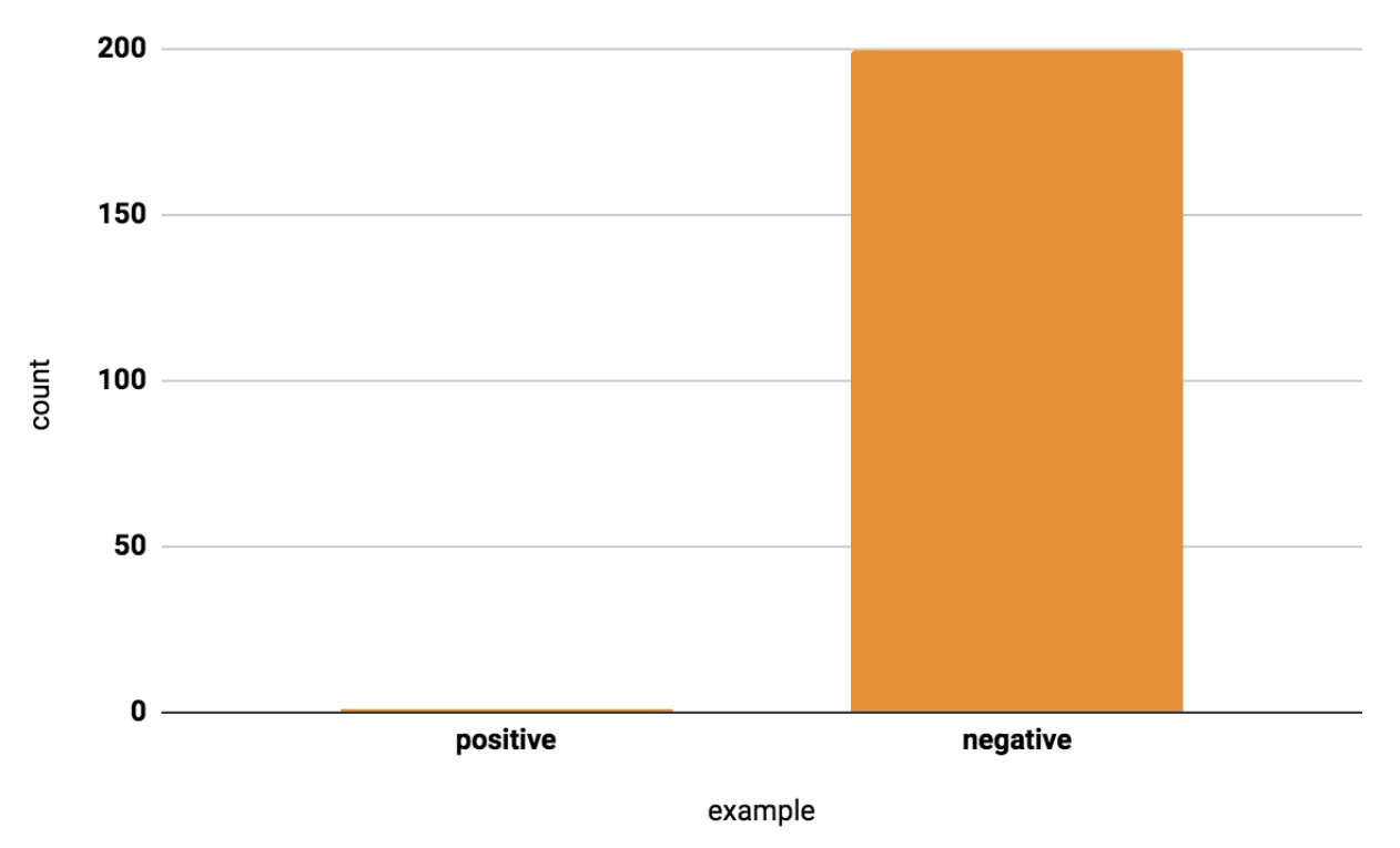
In supervised learning, a balanced dataset means that each class has approximately the same number of instances. An imbalanced dataset, conversely, is one where the classes are not represented equally. For instance, in a binary classification problem, you might have 90% of samples labeled as 'Class A' and only 10% labeled as 'Class B'. Such imbalances can lead to significant issues; for example, a machine learning model trained on this data could become biased toward 'Class A', producing predictions that are highly skewed and possibly misleading.

Why It Matters
The risk of working with imbalanced datasets is that the model you train will likely become biased, favoring the majority class. It may simply learn to always predict 'Class A' and achieve high accuracy because 'Class A' is what it predominantly sees during training. This undermines the model's utility, as it may fail to correctly identify instances of the minority class, which could be critical in applications like fraud detection, medical diagnosis, or any other domain where the minority class is more impactful or costly.
Resampling Techniques
There are several methods to mitigate the issues caused by imbalanced datasets, one of the most straightforward being resampling. Resampling methods are categorized into:
Upsampling the Minority Class: This involves randomly replicating instances from the minority class in the training dataset. Although effective, the downside is that it can lead to overfitting since it doesn't introduce any new information, only duplicates existing samples.
Downsampling the Majority Class: Here, random instances from the majority class are removed until balance is restored. While this method can improve the model's performance on the minority class, it also removes potentially useful data.
Synthetic Data Generation
Another sophisticated approach is synthetic data generation, most commonly done using the Synthetic Minority Over-sampling Technique (SMOTE). SMOTE works by selecting samples that are close in the feature space, drawing a line between the samples in the feature space, and generating new samples at points along that line. This technique helps to combat the overfitting problem that can occur with simple upsampling.
Algorithmic Approach
An alternative to modifying the dataset is to adapt the algorithm used for training to be more sensitive to the minority class. Many machine learning algorithms offer hyperparameters that can be tuned to adjust the weight given to each class. For example, in scikit-learn's implementation of logistic regression, you can use the class_weight parameter to specify a higher penalty for misclassifying the minority class.
Evaluation Metrics
Finally, it's crucial to evaluate the model's performance using metrics designed to give insights into class distribution, such as the F1-score, precision-recall curves, or the area under the Precision-Recall curve (AUC-PR), instead of relying solely on accuracy.
Handling imbalanced datasets requires thoughtful consideration and a mix of techniques. Understanding the trade-offs between different approaches will allow you to develop a more robust and reliable machine learning model.
Conclusion
In this week's post, we've covered some advanced techniques that can help enhance the performance and reliability of your supervised learning models. We explored ensemble methods to combine the predictions from multiple models, discussed regularization techniques to prevent overfitting, and offered strategies for handling imbalanced datasets.
These advanced techniques serve as tools in your machine learning toolbox, allowing you to adapt and improve your models based on specific challenges you may encounter.
As always, the key to mastering these methods lies in practice. I encourage you to implement these techniques in your own projects and observe the impact they have on model performance.
In the coming weeks, we will venture into other exciting areas of machine learning.
Thank you for following along, and happy coding!
References
https://scikit-learn.org/stable/modules/classes.html#module-sklearn.linear_model


