
Mastering Hyperparameter Optimization
Unlocking the Full Potential of Supervised Learning Models with Python


Introduction
In the ever-evolving landscape of machine learning, deploying a basic model is often just the starting point. As we've previously discussed and demonstrated, scikit-learn provides an accessible platform for implementing a wide variety of algorithms. However, your journey towards developing a high-performing model doesn't stop once you've picked an algorithm and fit it to your data. This brings us to the objective of this week's blog post: delving into the intricate world of fine-tuning and hyperparameter optimization.
Hyperparameters are parameters whose values are set before the learning process begins, unlike the internal parameters that the model learns through training. Examples include the learning rate in gradient boosting or the regularization term in a support vector machine. The task of finding the optimal set of hyperparameters is both an art and a science, often requiring a careful balance between computational efficiency and model performance.
Why is hyperparameter optimization so essential? The reason is twofold. First, it allows you to extract the maximum predictive power from your models. Even minor adjustments can lead to significant performance gains, impacting metrics such as accuracy, precision, and recall. Second, optimized hyperparameters can make your models more robust, generalizing better to new, unseen data. This is crucial for real-world applications where the cost of a poor prediction can be high.
In this blog post, we'll explore techniques for hyperparameter optimization like Grid Search, Random Search, and Bayesian Optimization. We'll walk through code examples that illustrate how to fine-tune your models using these optimizations along with a scikit-learn classifier, and then evaluate the impact of these adjustments. By the end, you'll have a robust toolkit for elevating your supervised learning models from good to great.
Techniques for Hyperparameter Optimization
Hyperparameter optimization is an indispensable step in the machine learning pipeline, and its importance cannot be overstated. While model parameters are learned during the training process, hyperparameters are external configurations for the algorithm that are not learned from the data. These could include learning rates, regularization terms, or the number of hidden layers in a neural network, among others. The process of finding the optimal hyperparameters for your model can substantially improve the model's performance. In this post, we will delve into the intricacies of hyperparameter optimization, discuss different techniques, and show how these can be implemented.
Techniques for Hyperparameter Optimization
Grid Search
The most straightforward method for hyperparameter optimization is Grid Search. In this technique, you define a grid of hyperparameters and evaluate model performance for each point on the grid. You then select the point that gives the best performance based on a scoring metric like accuracy or F1-score. Although grid search is simple to understand and implement, it can be computationally expensive as the number of hyperparameters grows, leading to an exponential increase in the number of combinations to test.
Here's how to implement Grid Search using scikit-learn:
from sklearn.model_selection import GridSearchCV
from sklearn.svm import SVC

# Define the parameter grid
param_grid = {
    'C': [0.1, 1, 10],
    'kernel': ['linear', 'rbf']
}

# Initialize the model
svc = SVC()

# Initialize Grid Search
grid_search = GridSearchCV(estimator=svc, param_grid=param_grid, cv=5)

# Fit the model
grid_search.fit(X_train, y_train)

# Get the best parameters
best_params = grid_search.best_params_
Random Search
An alternative to Grid Search is Random Search, where random combinations of the hyperparameters are used to find the best solution. While this may sound inefficient, studies have shown that Random Search can be more efficient than Grid Search, especially when the number of hyperparameters is large. It's generally faster and can converge to the optimal set of hyperparameters quicker because it samples a broader range of values.
Here's a sample code snippet for implementing Random Search in scikit-learn:
from sklearn.model_selection import RandomizedSearchCV

# Define the parameter grid
param_dist = {
    'C': [0.1, 1, 10],
    'kernel': ['linear', 'rbf']
}

# Initialize Random Search
random_search = RandomizedSearchCV(SVC(), param_distributions=param_dist, n_iter=10, cv=5)

# Fit the model
random_search.fit(X_train, y_train)

# Get the best parameters
best_params = random_search.best_params_
Bayesian Optimization
Bayesian Optimization is a probabilistic model-based optimization technique. Unlike Grid Search and Random Search, Bayesian Optimization takes into account past evaluations to select the next hyperparameters to evaluate. This results in a more intelligent search across the hyperparameter space, usually requiring fewer evaluations to find the optimal set.
Implementing Bayesian Optimization can be a bit more involved, but libraries like scikit-optimize can make it easier. With Bayesian Optimization, you usually define a function to optimize, in this case, the validation score, and then run the optimization algorithm to maximize this function. We will walk through a code example of this in the next section.
Hyperparameter optimization is an essential yet often overlooked aspect of model development. The techniques discussed here—Grid Search, Random Search, and Bayesian Optimization—offer a good starting point for practitioners aiming to improve model performance. While Grid Search is a good choice for lower-dimensional hyperparameter spaces, Random Search and Bayesian Optimization offer more efficient alternatives for high-dimensional spaces. These techniques can be easily implemented in Python using the scikit-learn library, allowing you to fine-tune your models and achieve superior performance.
Code Walkthrough: Bayesian Hyperparameter Optimization
As we covered, Bayesian Optimization is a probabilistic model-based optimization technique aimed at finding the minimum of any function that returns a real-value metric. It is particularly well-suited for optimizing complex, high-dimensional functions that are expensive to evaluate. In machine learning, it can be used for hyperparameter tuning, effectively replacing grid search and random search methods. Today, we'll see how to apply Bayesian Optimization to optimize the hyperparameters of a RandomForestClassifier using the bayes_opt library.
The Setup
First, let's complete the code setup. We have the run_classifier function, which takes in a classifier and returns the mean and standard deviation of accuracy, as well as the mean True Positive Rate (TPR) and False Positive Rate (FPR). This function uses 10-fold stratified cross-validation.
from sklearn.metrics import accuracy_score, confusion_matrix
from sklearn.model_selection import StratifiedKFold
from sklearn.ensemble import RandomForestClassifier
import numpy as np

bop_log = []

def run_classifier(classifier, log_progress=False):
    global feature_data, target_data, bop_log
    X_data, y_data = feature_data, target_data
    true_positive_rates = []
    false_positive_rates = []
    accuracies = []

    kfold = StratifiedKFold(n_splits=10, shuffle=True, random_state=0)

    for train_indices, test_indices in kfold.split(X_data, y_data):
        classifier.fit(X_data[train_indices], y_data[train_indices])
        y_predicted = classifier.predict(X_data[test_indices])

        acc = accuracy_score(y_data[test_indices], y_predicted)
        accuracies.append(acc)

        tn, fp, fn, tp = confusion_matrix(y_data[test_indices], y_predicted, labels=[1, 0]).ravel()

        true_positive_rate = tp / (tp + fn)
        false_positive_rate = fp / (fp + tn)

        true_positive_rates.append(true_positive_rate)
        false_positive_rates.append(false_positive_rate)

    mean_tpr = np.mean(true_positive_rates)
    mean_fpr = np.mean(false_positive_rates)

    if log_progress:
        bop_log.append((mean_tpr, mean_fpr))

    return np.mean(accuracies), np.std(accuracies), mean_tpr, mean_fpr
The costf function is our objective function that we aim to maximize. It takes in hyperparameters for the Random Forest Classifier and returns the cost.
# You may require this package install via pip or other package managers
from bayes_opt import BayesianOptimization

def avg(_x):
    return (_x[0]+_x[1])/2.

def costf(_X):  # BOP maximizes
    def costf(_pd, _pf):
        return 5*(1.-_pd)+_pf

    S = _X.shape[0]  # number of particles
    costs = np.ones((S,), dtype=float)

    for i in range(S):
        hp = np.array(_X[i], int)  # hyperparameters are integers
        clf = RandomForestClassifier(n_estimators=hp[0], max_depth=hp[1], max_features=hp[2], n_jobs=-1)
        acc, std, tpr, fpr = run_classifier(clf, log_progress=True)
        costs[i] = costf(tpr, fpr)

    return costs
Let's start by creating some random test data (X_train, y_train) that we'll use for our example.
from sklearn.datasets import make_classification

# Create random data
feature_data, target_data = make_classification(n_samples=1000, n_features=20, n_informative=15, n_redundant=5)
Define Hyperparameter Bounds
Before we run the Bayesian Optimization, let's set the bounds for the hyperparameters we are interested in tuning. For the Random Forest Classifier, we'll be tuning:
Number of estimators (
ne)Maximum depth (
md)Maximum features (
mf)
# Define the bounds for the hyperparameters
N_ESTIM = (10, 20)
MAX_DEP = (1, 10)
MAX_FEA = (1, 5)

pbounds = {'ne': N_ESTIM, 'md': MAX_DEP, 'mf': MAX_FEA}
The Objective Function for Bayesian Optimization
The function costf_bop is what the Bayesian Optimization will maximize. It's a wrapper around costf, converting the hyperparameters and preparing them for costf.
def costf_bop(ne, md, mf):  # Bayesian Op maximizes
    cost = costf(np.array([ne, md, mf]).reshape(-1, 3))
    return -cost[0]
Running the Bayesian Optimization
Now, let's set up and run the Bayesian Optimization.
from bayes_opt import BayesianOptimization

# Initialize Bayesian Optimization
boptim = BayesianOptimization(
    f=costf_bop,
    pbounds=pbounds,
    random_state=0,
)

PSO_ITERS_N = 20  # Number of iterations
bop_log = []  # collect Pd Pf

# Run the optimizer
boptim.maximize(init_points=3, n_iter=PSO_ITERS_N)
This shows the following output (note that it is a stochastic process so your results may not match):
|   iter    |  target   |    md     |    mf     |    ne     |
-------------------------------------------------------------
| 1         | -1.176    | 5.939     | 3.861     | 16.03     |
| 2         | -1.212    | 5.904     | 2.695     | 16.46     |
| 3         | -1.299    | 4.938     | 4.567     | 19.64     |
| 4         | -0.9851   | 6.335     | 4.362     | 14.41     |
| 5         | -1.021    | 6.657     | 4.995     | 13.04     |
| 6         | -0.9366   | 8.014     | 2.924     | 13.4      |
| 7         | -1.274    | 6.094     | 1.373     | 11.92     |
| 8         | -0.8495   | 8.978     | 4.4       | 14.27     |
| 9         | -0.9305   | 10.0      | 2.504     | 15.18     |
| 10        | -0.7693   | 10.0      | 4.455     | 12.17     |
| 11        | -0.9965   | 9.906     | 4.04      | 10.15     |
| 12        | -0.897    | 9.877     | 3.037     | 12.77     |
| 13        | -0.7746   | 10.0      | 5.0       | 13.32     |
| 14        | -2.036    | 1.0       | 5.0       | 10.0      |
| 15        | -0.915    | 10.0      | 1.0       | 20.0      |
| 16        | -0.8546   | 9.821     | 4.994     | 19.86     |
| 17        | -1.63     | 1.0       | 1.0       | 20.0      |
| 18        | -0.7748   | 10.0      | 5.0       | 17.25     |
| 19        | -0.8326   | 9.987     | 3.002     | 18.62     |
| 20        | -0.9345   | 10.0      | 1.0       | 17.53     |
| 21        | -0.817    | 10.0      | 5.0       | 11.81     |
| 22        | -0.6787   | 10.0      | 5.0       | 15.64     |
| 23        | -0.8071   | 9.962     | 4.245     | 16.27     |
=============================================================
Results and Best Parameters
After the optimization is complete, let's look at the best parameters and costs.
print(f"cost= {boptim.max['target']:.3f}")
bop_op_params = [int(boptim.max['params']['ne']), int(boptim.max['params']['md']), int(boptim.max['params']['mf'])]
print(f"OP params= {bop_op_params}")

# best OP
_, _, bop_tpr, bop_fpr = run_classifier(
    RandomForestClassifier(n_estimators=bop_op_params[0],
                           max_depth=bop_op_params[1], max_features=bop_op_params[2], n_jobs=-1))

Fpr1, Tpr1 = [_[1] for _ in bop_log], [_[0] for _ in bop_log]
Std1 = 0.02*np.ones((len(Tpr3),), dtype=float)
which outputs:
cost= -0.679
OP params= [15, 10, 5]
Meaning our number of estimators, max depth and max features were optimized to be: 15, 10, and 5, respectively.
ROC Curve
Finally, let's plot the Receiver Operating Characteristic (ROC) curve to visualize the performance.
import matplotlib.pyplot as plt

def plotr(_ax, _fpr, _tpr, _std0, _label, op=None):
    _ax.scatter(_fpr, _tpr, s=_std0 * 1000, marker='o', c='r', edgecolors='k', alpha=0.8, label=_label)
    if op is not None:
        _ax.scatter(op[0], op[1], s=50, marker='d', c='b', label='OP')
    _ax.plot(np.arange(0.001,1,0.01), np.arange(0.001,1,0.01), linestyle='--', color=(0.6, 0.6, 0.6), label='coin flip')
    _ax.set(xlabel='False Positive Rate', ylabel='True Positive Rate')
    _ax.grid()
    _ax.legend()

_, ax = plt.subplots(1, 1, figsize=(10, 6), dpi=72)

Fpr1, Tpr1 = [_[1] for _ in bop_log], [_[0] for _ in bop_log]
Std1 = 0.02*np.ones((len(Tpr1),), dtype=float)

print(Fpr1)
print(Tpr1)

plotr(ax, Fpr1, Tpr1, Std1, 'Bayesian Optimization', op=(bop_fpr, bop_tpr))

plt.show()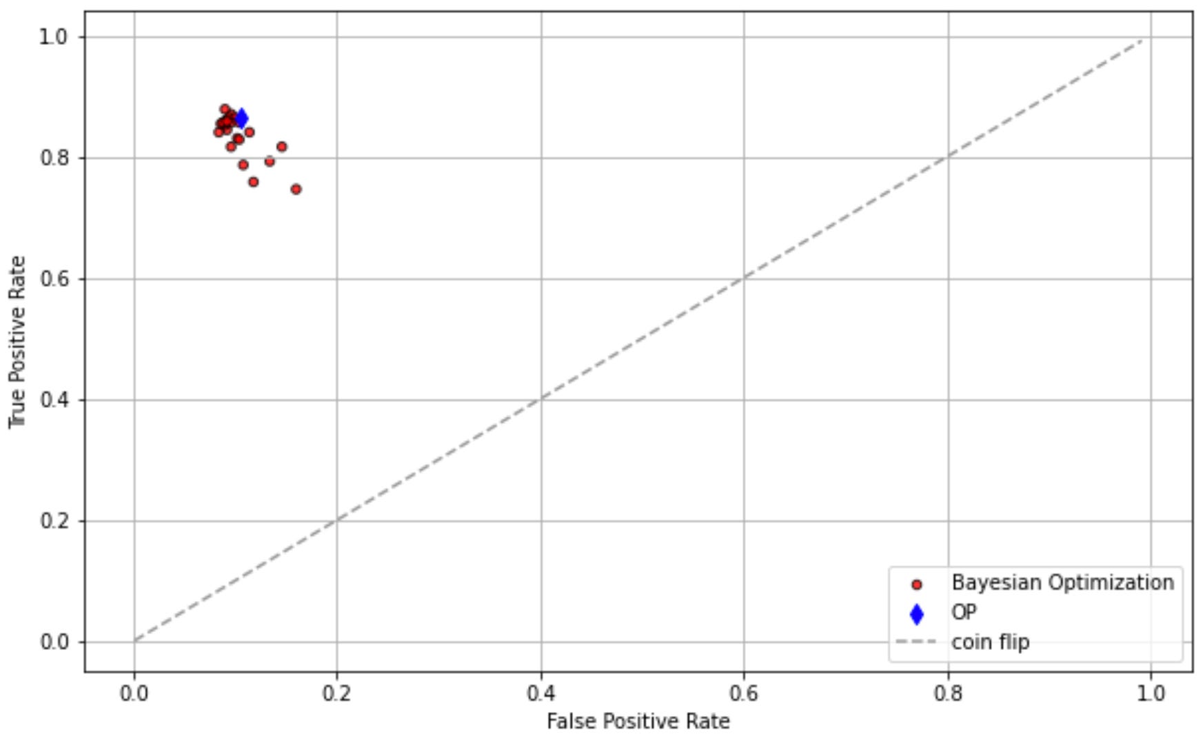
And there you have it! This is a simple but effective demonstration of how Bayesian Optimization can be applied for hyperparameter tuning in machine learning models. Happy tuning!
Evaluating the Impact
After the labor-intensive process of hyperparameter optimization, it's crucial to assess the impact of these changes on your models. It's not enough to merely tweak parameters; the real test of their efficacy comes from a comprehensive performance evaluation. Here, we'll explore how to compare model performance before and after hyperparameter tuning to determine the tangible benefits (or drawbacks) of the optimization process.
Baseline Performance Metrics
The first step in evaluating the impact of hyperparameter tuning is to establish a baseline for comparison. Before starting the tuning process, one should note down the performance metrics of the model on both training and test datasets. This can be accomplished using scikit-learn's built-in metrics functions for classification and regression problems, such as accuracy_score, precision_score, recall_score, and f1_score for classification tasks, or mean_absolute_error and mean_squared_error for regression tasks. These baseline metrics serve as a point of reference, allowing you to quantify the improvements (or deteriorations) in model performance post-optimization.
Performance Metrics Post-Tuning
Once you've undergone the hyperparameter tuning process—be it through grid search, random search, or Bayesian optimization—it's time to re-evaluate your models using the same performance metrics. Make sure to perform this evaluation on the same test dataset to ensure that any changes in performance can be attributed to the hyperparameter tuning rather than variations in the data.
Comparative Analysis
With baseline and post-tuning metrics in hand, the next step is a comparative analysis. One straightforward approach is to calculate the percentage improvement for each performance metric. For example, if the baseline accuracy was 80%, and the post-tuning accuracy jumps to 85%, that represents a 5% improvement. However, the utility of an improvement also depends on the specific application. In some fields like healthcare or finance, even a modest percentage improvement could have a substantial real-world impact.
Visual Representation
Sometimes, numbers alone can't capture the full story. Visual representations such as line graphs or bar charts comparing the before-and-after metrics can make the improvements more intuitive and easier to grasp. These visual aids can be particularly useful when presenting your findings to an audience that may not be as familiar with machine learning terminology and metrics.
Contextualizing the Improvements
It's also essential to contextualize these improvements in the broader scope of your project or application. Is the percentage improvement in performance metrics meaningful in terms of business objectives? Does it translate to better user experience, higher sales, or more accurate predictions? Sometimes, a smaller improvement in a critical metric could be more valuable than a large improvement in a less important one.
Limitations and Trade-offs
Lastly, it's critical to acknowledge any limitations and trade-offs that come with hyperparameter tuning. For instance, a more complex model may perform better but could be computationally expensive and harder to deploy. Or, tuning a model for higher precision might result in lower recall, depending on the problem at hand. Being transparent about these trade-offs helps set realistic expectations and aids in making informed decisions for project stakeholders.
In summary, evaluating the impact of hyperparameter tuning involves a multi-faceted approach that goes beyond merely reporting the change in performance metrics. By comprehensively analyzing and contextualizing these changes, you can offer a nuanced understanding of the real-world implications of your optimization efforts.
Conclusion
In wrapping up this week's exploration into the art and science of hyperparameter optimization, we've unearthed the critical role that fine-tuning plays in the performance of supervised learning models. We delved into various techniques, from Grid Search to Bayesian Optimization, and showcased how even small adjustments can result in substantial improvements. The tangible gains in accuracy, precision, or recall, depending on your specific use-case, demonstrate that model tuning is not a mere academic exercise but a necessary step in the pipeline of any serious machine learning project. As we move forward, we'll delve into more advanced topics that will help us become not just practitioners but experts in the field. Stay tuned for next week as we explore the intriguing world of ensemble methods, which offer yet another avenue for improving model performance.
I hope this week's post has added another layer to your understanding of supervised learning. As always, the code used in the examples is available in the linked GitHub repository for further exploration. Thank you for joining me on this journey, and I look forward to guiding you through more advanced topics in our upcoming installment.
GitHub Code
You can find the complete Jupyter Notebook containing all the code, explanations, and visualizations covered in this post on GitHub.